Exam - R programming

Chicago Crimes from 2019 to 2021

Ariz WEBER - Nathan PIZZETTA

December 2023

Formating the output

# Format of our datatables
styled_dt <- function(df, n=5) {DT::datatable(df, 
                                        extensions = 'Buttons',
                                        rownames = FALSE,
                                        options = list(
                                          scrollX = TRUE, 
                                          pageLength = n,
                                          dom = 'Bfrtip',
                                          buttons = c('copy', 'csv', 'excel')
                                          ))}

Import of our datasets

setwd("/Users/nathanpizzetta/Documents/TSE/Cours/M1/Software for Data Science/R/exam")

df19 <- read.csv("Crime_Chicago_2019.csv")
df20 <- read.csv("Crime_Chicago_2020.csv")
df21 <- read.csv("Crime_Chicago_2021.csv")

Chicago crimes

styled_dt(df19[1:500, ])

styled_dt(df20[1:500, ])

styled_dt(df21[1:500, ])

Tidying and basing our datasets

# Basing our datasets
df <- bind_rows(df19, df20)
df <- bind_rows(df, df21)

Here by plotting “df” which is our big dataset, we can see that some columns are not common to the three datasets. We therefore chose not to keep them because they will not be useful. Also, we see that for the location we got three columns. We choose to keep only the columns “Longitude” and “Latitude”.

To drop this columns we will use select.

# Droping the columns we do not want
df <- select(df, c(Case.Number, Date, Arrest, District, Year, Latitude, Longitude))

# We add a new column for months which will be usefuk to us
df$Date <- lubridate::parse_date_time(df$Date, "%m/%d/%y %I:%M:%S %p")
df$Month <- month(df$Date)
df$Day <- day(df$Date)
df$Wday <- as.POSIXlt(df$Date)$wday
df$Hour <- hour(df$Date)

styled_dt(df[1:500, ])

Taking a look to the crimes

count_df <- df %>% group_by(Year, Month) %>% count()
count_df$Date<- zoo::as.Date(with(count_df,paste(Year,Month,sep="-")), "%Y-%m")
count_df$Date <- zoo::as.yearmon(with(count_df,paste(Year,Month,sep="-")))

# Plot
count_df_plot <- count_df[,c("Date", "n")]
dygraphs::dygraph(data=count_df_plot, main="Crime Count per MONTH", ylab="crime count")

count_df_day <- df %>% group_by(Year, Month, Day) %>% count()
count_df_day$Date<- as.Date(with(count_df_day,paste(Year,Month,Day,sep="-")), "%Y-%m-%d")
count_df_plot <- count_df_day[,c("Date", "n")]

# Plot
dygraphs::dygraph(data=count_df_plot, main="Crime Count per Day", ylab = "crime count")

df$District <- as.factor(df$District)

# Plot
ggplot(data = df, aes(x = District)) +
  geom_histogram(stat = "count") +
  ylab("crime count") +
  xlab("District") + 
  ggtitle("Crime count per District")

Warning in geom_histogram(stat = "count"): Ignoring unknown parameters:
`binwidth`, `bins`, and `pad`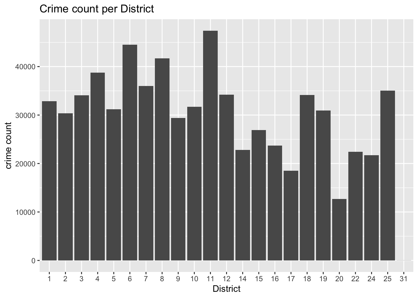

# Plot
ggplot(data = df, aes(x = Hour)) +
  geom_histogram(bins=24, binwidth = 0.5) +
  ylab("crime count") +
  xlab("Hour of the day") +
  ggtitle("Crime count per Hour of Day")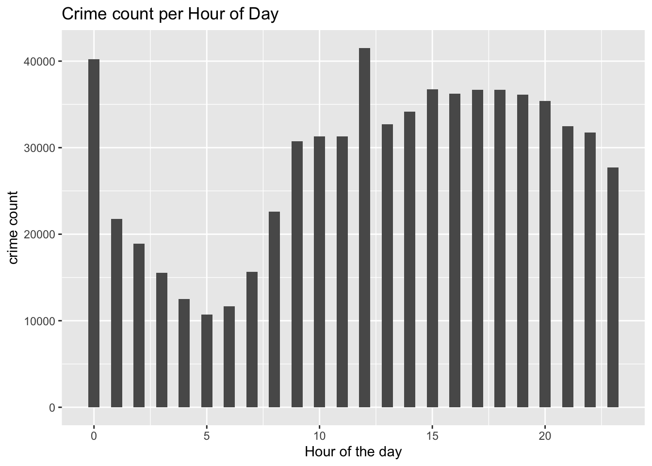

Crimes on May the 31^st of 2020

# Filtering on a specific month
may_2020_31 <- df %>% dplyr::filter(Year == 2020, Month == 5, Day == 31, !is.na(Latitude))


# Map
mapview::mapview(may_2020_31, xcol = "Longitude", ycol = "Latitude", crs = 4269, grid = FALSE, layer.name ="Crime")